While Gradient Descent isn’t traditionally thought of as a machine-learning algorithm, understanding gradient descent is vital* *to understanding how many machine learning algorithms work and are optimized. Understanding Gradient Descent might require a brief knowledge of Calculus, but I have tried my best to keep it as simple as possible.

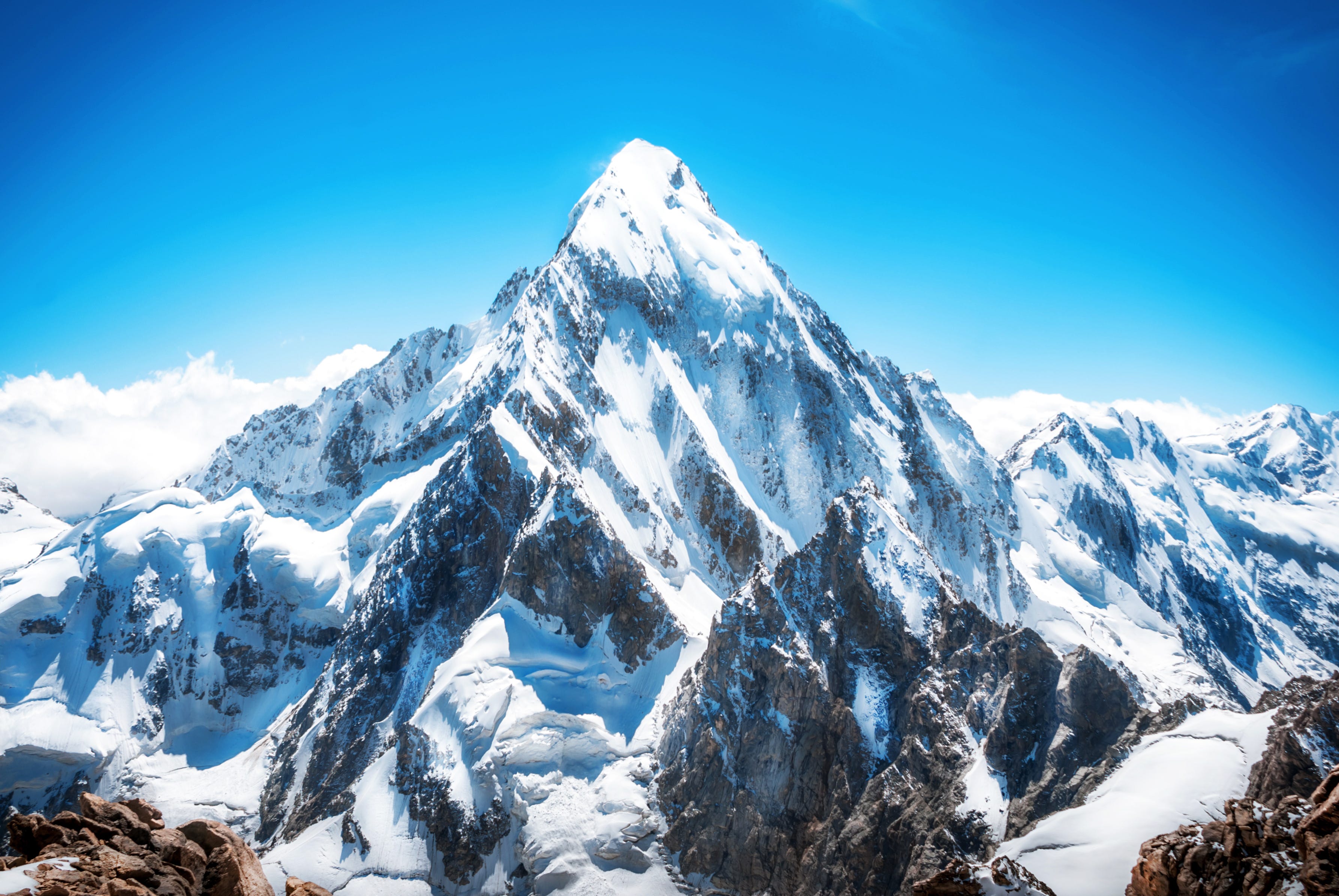
Before we see the definition of Gradient descent let us try to break the words and understand what it actually means. Gradient means an inclined part of a pathway or a slope, descent means to move towards the bottom of the slope. Imagine yourself to be a mountaineer and you are trying to get to the bottom of the mountain i.e. you are descending the gradient of the mountain. Let us for now just keep this in the back of our minds, we will revisit this example later.

---

Gradient Descent

Gradient descent is an optimization algorithm that’s used when training a machine learning model. It’s based on a convex function and tweaks its parameters iteratively to minimize a given function to its local minimum.

Gradient descent in simple words is used to find the values of a function’s parameters that minimize a cost function as far as possible.

You start by defining the initial parameter’s values and from there gradient descent uses calculus to iteratively adjust the values so they minimize the given cost-function.

---

Formula for Gradient Descent

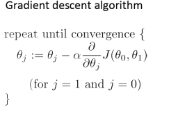
Here θ0 and θ1 are parameters of cost function J(θ0, θ1). ‘α’ is the learning rate of the gradient descent which decides the length of steps taken towards minimum. The partial derivative term tells the direction of the steepest descent.

Now, lets go back to the example where you were imagining to be a mountaineer, dreaming to reach the bottom most point of the mountain. Imagine the parameters defining the position of mountaineer, the learning rate defining the rate at which mountaineer descends the mountain and the partial derivative term defining the path to be taken to reach the bottom most point (minimum). The objective is to reach the bottom most point of the mountain i.e. the minimum.

---

How Gradient Descent Works?

Imagine you have a machine learning problem and want to train your algorithm with gradient descent to minimize your cost-function J(θ0, θ1) and reach its local minimum by tweaking its parameters (θ0 and θ1). The image below shows the horizontal axes represent the parameters (θ0 and θ1), while the cost function J(θ0, θ1) is represented on the vertical axes. The Illustration explains the working of Gradient Descent.

We know we want to find the values of θ0 and θ1 that correspond to the minimum of the cost function. To start finding the right values we initialize θ0 and θ1 with some random numbers. Gradient descent then starts at that point (somewhere around the top of our illustration), and it takes one step after another in the steepest downside direction (i.e., from the top to the bottom of the illustration) until it reaches the point where the cost function is as small as possible.

In the given example, the cost function is non-convex, but for most Machine Learning problems, the cost functions are convex. For eg:

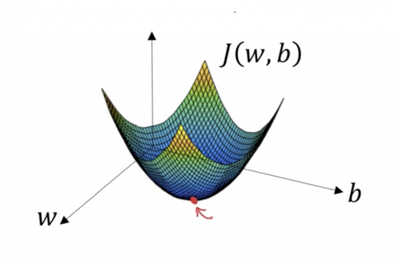
The red point marked is the minimum of the cost function. Thus, for any chosen value of the parameters, the minimum of the function would be same.

---

Importance of Learning Rate

Learning rate ‘α’ determines the length of the steps taken in the direction of local minimum, which figures out how fast or slow we will move towards the optimal weights. For gradient descent to reach local minimum its important to choose an appropriate value for learning rate. It should neither be too low or too high.

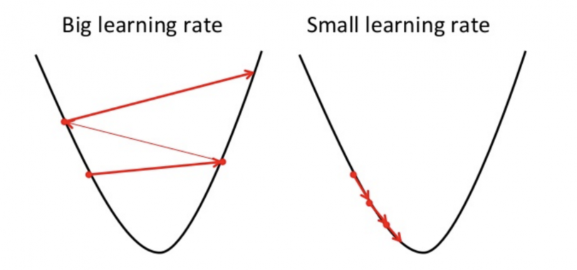
This is important because if the steps it takes are too big, it may not reach the local minimum because it bounces back and forth between the convex function of gradient descent. If we set the learning rate to a very small value, gradient descent will eventually reach the local minimum but that may take a while.

---

How to check Working of Gradient Descent

A good way to make sure gradient descent runs properly is by plotting the cost function as the optimization runs. Put the number of iterations on the x-axis and the value of the cost-function on the y-axis. This helps you see the value of your cost function after each iteration of gradient descent, and provides a way to easily spot how appropriate your learning rate is. You can just try different values for it and plot them all together.

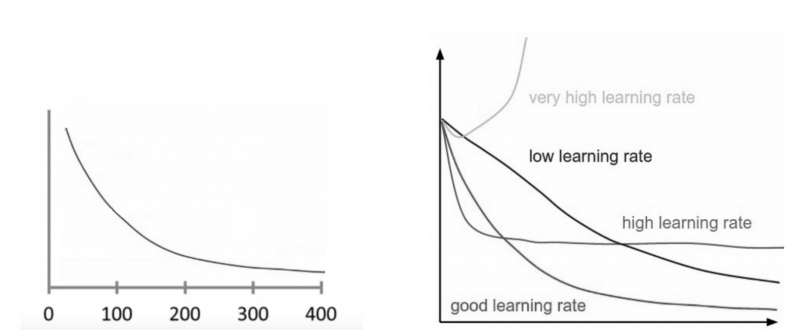
If gradient descent is working properly, the cost function should decrease after every iteration. When gradient descent can’t decrease the cost-function anymore and remains more or less on the same level, it has converged.

One advantage of monitoring gradient descent via plots is it allows us to easily spot if it doesn’t work properly, for example if the cost function is increasing. Most of the time the reason for an increasing cost-function when using gradient descent is a learning rate that’s too high.

---

Types of Gradient Descent

There are three popular types of gradient descent that mainly differ in the amount of data they use:

1. Batch Gradient Descent

In Batch Gradient Descent, all the training data is taken into consideration to take a single step. We take the average of the gradients of all the training examples and then use that mean gradient to update our parameters. So that’s just one step of gradient descent in one iteration.

Batch Gradient Descent is great for convex or relatively smooth error manifolds. In this case, we move somewhat directly towards an optimum solution.

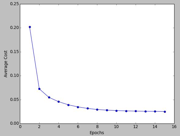
The graph of cost vs iterations (Epoch) is quite smooth. The cost keeps on decreasing over the iterations.

1. Stochastic Gradient Descent

In Batch Gradient Descent we were considering all the examples for every step of Gradient Descent. But what if our dataset is very huge. Suppose our dataset has 5 million examples, then just to take one step the model will have to calculate the gradients of all the 5 million examples. This does not seem an efficient way. To tackle this problem, we have Stochastic Gradient Descent. In Stochastic Gradient Descent (SGD), we consider just one example at a time to take a single step.

Since we are considering just one example at a time the cost will fluctuate over the training examples and it will **not **necessarily decrease. But in the long run, you will see the cost decreasing with fluctuations.

Also, because the cost is so fluctuating, it will never reach the minima but it will keep dancing around it. SGD can be used for larger datasets. It converges faster when the dataset is large as it causes updates to the parameters more frequently.

1. Mini Batch Gradient Descent

Mini-batch gradient descent is the go-to method since it’s a combination of the concepts of SGD and batch gradient descent. It simply splits the training dataset into small batches and performs an update for each of those batches. This creates a balance between the robustness of stochastic gradient descent and the efficiency of batch gradient descent.

Just like SGD, the average cost over the epochs in mini-batch gradient descent fluctuates because we are averaging a small number of examples at a time.

Common mini-batch sizes range between 50 and 256, but like any other machine learning technique, there is no clear rule because it varies for different applications. This is the go-to algorithm when training a neural network and it is the most common type of gradient descent within deep learning.

---

Conclusion

Gradient Descent is the heart of most machine learning problems. It’s important for us to know how these machine learning algorithms reach the optimal value. Here is an example of how Gradient Descent is used in Regression:

Just like every other thing in this world, all the three variants we saw have their advantages as well as disadvantages. It’s not like the one variant is used frequently over all the others. Every variant is used uniformly depending on the situation and the context of the problem.

---

About the author

Shrikumar Shankar, is an undergraduate pursuing B. Tech from SRM IST. He is an enthusiast in Machine Learning and loves to share the knowledge gained through his blogs. He aims to make non-tech people aware of the basic terminologies of machine learning and its applications.

---

Reviews

If You find it interesting!! we would really like to hear from you.

Ping us at Instagram/@the.blur.code

If you want articles on Any topics dm us on insta.

Thanks for reading!! Happy Coding