With the rise of machine learning frameworks, we can now train classifiers with just a few lines of code. For traditional machine learning applications (in case you’re wondering, Deep Learning is the not-so traditional thing I’m talking about), the library scikit-learn is very widely used. It’s very user friendly, comes with a lot of hyper-parameters to alter in case we don’t get a decent accuracy.

Metrics: Metre, Celsius, oh wait! The metrics are different here. Here are some of the metrics generally used to measure the performance of a classifier:

Accuracy: It is the simplest metric, that just returns the fraction of correctly classified labels to the total number of prediction. It’s easy to calculate and very widely used.

Accuracy

The next metrics are based on confusion matrix. Confusion matrix are based on 4 things:

1. True Positives: The labels that are correctly classified as positive by the classifier.
2. False Positives: The labels that are incorrectly classified as positive by the classifiers while they are negative in reality.
3. True negatives: The labels that are correctly classified as negative by the classifier.
4. False Negatives: The labels that are incorrectly classified as negative by the classifier while they are positive in reality.

Confusion Matrix:

Real Values	Positive	Negative
Classifier Values
Positive	True Positive	False Negative
Negative	False Negative	True Negative

Precision: It is measured by the fraction of positive predictions that the classifier correctly classified to the number of total positive predictions.

Recall: It is measured by the fraction of predictions that are classified as positive by the classifier to the number of total positive examples in reality.

The two metrics precision and accuracy are generally not used in their raw form as they don’t form a good basis of measurement. Here comes the next important metric, known as f1 score.

Accuracy can also be measured using confusion properties:

F1 score: It is the harmonic mean (progressions and series anyone?) of the precision and mean multiplied by 2.

Area under curve score: The area enclosed by the graph of true positive rate and false positive rate can be used as a metric to calculate the efficiency of the classifier.

Mean Squared Error: It is measured by calculation of the mean of the squared difference between the predicted value and the true value.

Additionally, scaling the data can help the classifiers sometimes. There maybe a column, like price that can vary from 0 to 1 million (maybe more). And there might be another column like the number of family members which almost always stays in double digits (nope, no freaky family is taken into consideration). In such a case, having the values of all the columns normalised between 0 to 1 (or maybe any other lower and upper value) can really help the classifier.

Ok, enough of these metrics and theory. Let’s move in to the real job.

It’s generally a good habit to include the generic libraries at the beginning of the notebook.

import pandas as pd
import numpy as np
import matplotlib.pyplot as plt
import seaborn as sb
from sklearn.model_selection import train_test_split
from sklearn.preprocessing import MinMaxScaler
from sklearn.metrics import accuracy_score, f1_score
plt.style.use('seaborn')

In case, you’re wondering about the plt.style.use(), feel free to google it. It’s a pretty interesting thing ;).

Let’s load the Dataset and initiate our dictionaries.

acc_dict=
f1_dict={}
url= 'https://raw.githubusercontent.com/SurajSarangi/Iris-Flower-Classification/master/iris.csv'
df=pd.read_csv(url)
df.index=df.index+1
df.head()

	sepal_length	sepal_width	petal_length	petal_width	species
1	5.1	3.5	1.4	0.2	setosa
2	4.9	3.0	1.4	0.2	setosa
3	4.7	3.2	1.3	0.2	setosa
4	4.6	3.1	1.5	0.2	setosa
5	5.0	3.6	1.4	0.2	setosa

Plotting the Graphs for the attributes, gives us these graphs.

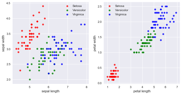
Setosa can be separated from the rest pretty easily by taking the petal length and petal width into account.

Now, the data is split into the training and test sets using the train_test_split. The data is then scaled using the MinMaxScaler.

cols=df.columns
X=df[cols[:-1]]
y=df[cols[-1]]
X_train,X_test,y_train,y_test=train_test_split(X,y,random_state=0)
X_train2=MinMaxScaler().fit_transform(X_train)
X_test2=MinMaxScaler().fit_transform(X_test)

Good News, the data is now ready for processing.

We’ll start with the most basic classifier. This would give us an idea of what is the baseline that we need to improve while training a classifier.

Naïve Bayes

from sklearn.naive_bayes import MultinomialNB

def mnb():
     mnb=MultinomialNB().fit(X_train,y_train)
     y_pred = mnb.predict(X_train)
     y_pred2= mnb.predict(X_test)
     s1 = accuracy_score(y_train, y_pred)
     s2 = f1_score(y_train, y_pred, average='macro')
     s3 = accuracy_score(y_test, y_pred2)
     s4 = f1_score(y_test, y_pred2, average='macro')
     acc_dict['Naive Bayes']=s3
     f1_dict['Naive Bayes']=s4
     return pd.DataFrame([[s1,s2],[s3,s4]], index=['Train','Test'], columns=['Accuracy','f1'])  

mnb()
 

	Accuracy	f1
Train	0.705357	0.590062
Test	0.578947	0.509804

Logistic Regression

from sklearn.linear_model import LogisticRegression

def lr2():
     lr=LogisticRegression(C=100, solver='lbfgs', multi_class='auto').fit(X_train2, y_train)
     y_pred = lr.predict(X_train2)
     y_pred2= lr.predict(X_test2)
     s1 = accuracy_score(y_train, y_pred)
     s2 = f1_score(y_train, y_pred, average='macro')
     s3 = accuracy_score(y_test, y_pred2)
     s4 = f1_score(y_test, y_pred2, average='macro')
     acc_dict['Logistic Regression (scaled)']= s3
     f1_dict['Logistic Regression (scaled)']= s4
     return pd.DataFrame([[s1,s2],[s3,s4]], index=['Train','Test'], columns=['Accuracy', 'f1'])
     
lr2()

	Accuracy	f1
Train	0.982143	0.982066
Test	0.973684	0.971703

We have significantly improved on our baseline. The parameters C, multi_class, solver are the hyper parameters. Tweaking them made it possible to achieve such scores. I’d advise you to try playing with them and maybe you can get a better score.

Decision Tree

from sklearn.tree import DecisionTreeClassifier

def dtr():
     dt=DecisionTreeClassifier().fit(X_train,y_train)
     y_pred = dt.predict(X_train)
     y_pred2= dt.predict(X_test)
     s1 = accuracy_score(y_train, y_pred)
     s2 = f1_score(y_train, y_pred, average='macro')
     s3 = accuracy_score(y_test, y_pred2)
     s4 = f1_score(y_test, y_pred2, average='macro')
     acc_dict['Decision Tree']= s3
     f1_dict['Decision Tree']= s4
     return pd.DataFrame([[s1,s2],[s3,s4]], index=['Train','Test'], columns=['Accuracy', 'f1'])

dtr() 

	Accuracy	f1
Train	1.000000	1.000000
Test	0.973684	0.971703

As we can see, Decision Tree achieves perfect scores on the training sets. However, it isn’t as brilliant when it comes to the test set. This problem is known as Overfitting. Using regularization is one good way to reduce overfitting. Tree algorithms generally tend to overfit the training data. Scaling the data will never help in case of trees.

Support Vector Machine

from sklearn.svm import SVC

def sv2():
     sv=SVC(C=0.7,kernel='rbf',gamma='scale').fit(X_train2,y_train)
     y_pred = sv.predict(X_train2)
     y_pred2= sv.predict(X_test2)
     s1 = accuracy_score(y_train, y_pred)
     s2 = f1_score(y_train, y_pred, average='macro')
     s3 = accuracy_score(y_test, y_pred2)
     s4 = f1_score(y_test, y_pred2, average='macro')
     acc_dict['SVM (scaled)']= s3
     f1_dict['SVM (scaled)']= s4
     return pd.DataFrame([[s1,s2],[s3,s4]], index=['Train','Test'], columns=['Accuracy', 'f1'])

sv2()

	Accuracy	f1
Train	0.973214	0.973026
Test	0.973684	0.971703

K Nearest Neighbours Classifier

from sklearn.neighbors import KNeighborsClassifier

def kn1():
    knn=KNeighborsClassifier(n_neighbors=16).fit(X_train,y_train)
    y_pred = knn.predict(X_train)
    y_pred2= knn.predict(X_test)
    s1 = accuracy_score(y_train, y_pred)
    s2 = f1_score(y_train, y_pred, average='macro')
    s3 = accuracy_score(y_test, y_pred2)
    s4 = f1_score(y_test, y_pred2, average='macro')
    acc_dict['kNN']= s3
    f1_dict['kNN']= s4
    return pd.DataFrame([[s1,s2],[s3,s4]], index=['Train','Test'], columns=['Accuracy', 'f1'])

kn1()

	Accuracy	f1
Train	0.964286	0.963925
Test	0.973684	0.971703

Random Forest

from sklearn.ensemble import RandomForestClassifier

def ran():
    rf=RandomForestClassifier(random_state=0).fit(X_train,y_train)
    y_pred = rf.predict(X_train)
    y_pred2= rf.predict(X_test)
    s1 = accuracy_score(y_train, y_pred)
    s2 = f1_score(y_train, y_pred, average='macro')
    s3 = accuracy_score(y_test, y_pred2)
    s4 = f1_score(y_test, y_pred2, average='macro')
    acc_dict['Random Forest']= s3
    f1_dict['Random Forest']= s4
    return pd.DataFrame([[s1,s2],[s3,s4]], index=['Train','Test'], columns=['Accuracy', 'f1'])

ran()

	Accuracy	f1
Train	1.000000	1.000000
Test	0.973684	0.971703

---

Multi layer Perceptron

It sounds like a name straight outta transformers! But this is our very own neural network. Yes, the most powerful classifier.

from sklearn.neural_network import MLPClassifier

def mlp():
    nn= MLPClassifier(hidden_layer_sizes=(10,10), solver='adam', random_state=0, alpha=0.1, max_iter=1000).fit(X_train, y_train)
    y_pred = nn.predict(X_train)
    y_pred2= nn.predict(X_test)
    s1 = accuracy_score(y_train, y_pred)
    s2 = f1_score(y_train, y_pred, average='macro')
    s3 = accuracy_score(y_test, y_pred2)
    s4 = f1_score(y_test, y_pred2, average='macro')
    acc_dict['Neural Network']= s3
    f1_dict['Neural Network']= s4
    return pd.DataFrame([[s1,s2],[s3,s4]], index=['Train','Test'], columns=['Accuracy', 'f1'])

mlp()

	Accuracy	f1
Train	0.982143	0.981962
Test	0.973684	0.971703

Now, you can laugh as to what on earth did the most powerful classifier achieve over the others. But, let me just tell you, that iris dataset is a really small dataset, with only 4 attributes, all of which are numerical. And as you can see, Neural Network has the maximum number of hyperparameters. Other classifiers may have a lot of hyperparameters, but none would match the usefulness and the efficiency of a Neural Network. Go ahead, feel free to have your own personal favourite classifier 

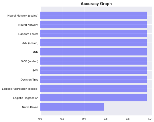
Score Graphs

Accuracy Graph:

plt.figure(figsize=(7,7))
plt.barh(range(len(acc_dict)), list(acc_dict.values()), align='center',color='blue',alpha=0.4,edgecolor='blue')
plt.yticks(range(len(acc_dict)), list(acc_dict.keys()))
plt.title('Accuracy Graph on Test', fontweight='bold', fontsize=14)
plt.show()

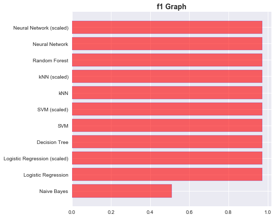
f1 Graph:

plt.figure(figsize=(7,7))
plt.barh(range(len(f1_dict)), list(f1_dict.values()), align='center',color='red',alpha=0.6,edgecolor='blue')
plt.yticks(range(len(f1_dict)), list(f1_dict.keys()))
plt.title('f1 Graph', fontweight='bold', fontsize=14)
plt.show()

These were some of the most widely used Classifiers. Hyperparameters are generally very important in getting good scores. Due to proper tuning of the hyperparameters, we could achieve similar scores from all the classifiers. If all these classifiers are invoked with the default values, then all these classifiers will give much different scores than what we have seen. Everyone has a favourite classifier. What would be yours?

Check out this link for the full notebook of this classification: https://github.com/SurajSarangi/Iris-Flower-Classification/blob/master/Iris.ipynb

---

About the author

Suraj Sarangi, is an undergrad, pursuing a degree in BTech. Python and Deep Learning are his weapons of choice. He is well versed in the language of English, likes to debate. Apparently, he loves football and coffee more than anything in his life.

---

Reviews

If You find it interesting!! we would really like to hear from you.

Ping us at Instagram/@the.blur.code

If you want articles on Any topics dm us on insta.

Thanks for reading!! Happy Coding